Text Segmentation is a task in Natural Language Processing that aims to divide a text document into semantically or topically coherent sections. This is useful for creating topic-specific summaries, organising long documents into sections for ease of reading, reducing noise, improving information retrieval, or to perform semantic chunking for Retrieval Augmented Generation (RAG), etc.
The goal of the task is to identify breakpoints between pairs of sentences where the topic deviates significantly. It is not necessary to know the number or identities of the topics themselves beforehand, and classifying the derived segments into meaningful categories can be done as a later step.
Text Segmentation based on semantics was first described in the TextTiling paper as an unsupervised learning task. Although it is possible to build a supervised model with sufficient training data, doing so requires additional effort for data annotation, and the model may suffer from domain overfitting. Therefore, in this post, we will focus on the unsupervised approach, which is more robust to various document types and domains.
This type of semantic segmentation is distinct from sentence boundary disambiguation, as we are not concerned with the syntactic structure of text, but rather the topical changes within it.
This approach is also applicable to spoken text directly. Human conversations, however, have other cues that can define a topic shift, such as pauses, changes in tone, or pitch. This technique cannot leverage such cues directly as it only uses lexical information to identify boundaries, but it could potentially do so with some modifications.
The algorithm
This technique operates by running a sliding window over sentences in the input text and calculating similarity scores between adjacent windows. Post-processing is then performed on these scores to extract boundary candidates to split the document.
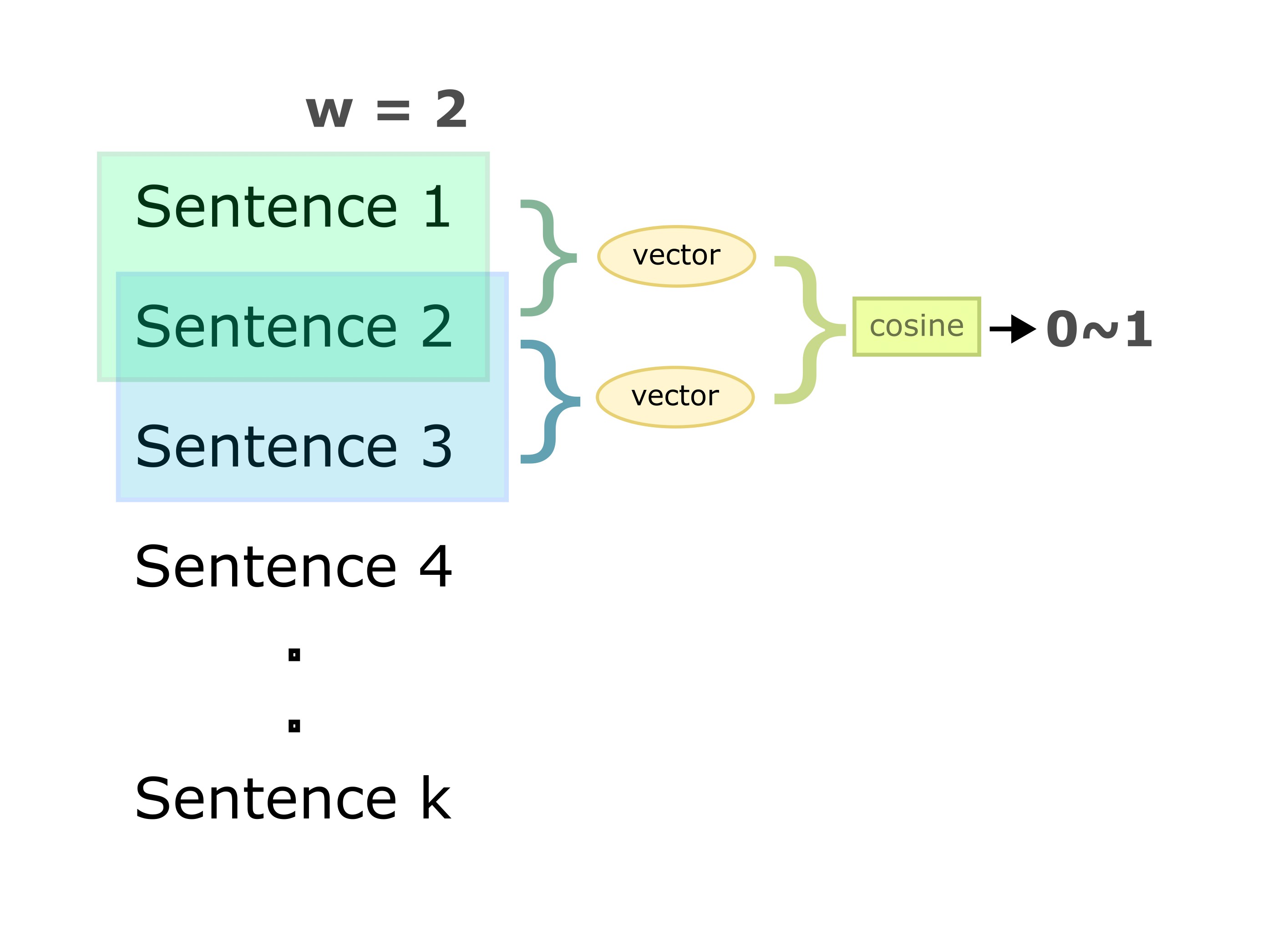
The scores can be calculated using a text similarity function that takes two pieces of text as an input and returns a score between 0 and 1. This function can be based on cosine similarity between bag-of-word features, topics derived from LDA, Word2Vec, large language models like BERT, etc.
In the next sections, we will implement the above algorithm to perform topic segmentation on a news article from the internet.
Preliminary Steps
We will use a Washington Post article as a sample document. I copied the text content and put it into a file called sample.txt where the paragraphs are separated by newlines.
Loading the Text
We can read the file using the following code, texts is a list containing the paragraphs in the document.
with open('input/sample.txt') as f:
	texts = f.read().splitlines()
The paragraphs need to be segmented into sentences, and each sentence has to be tokenised into words to carry out later steps. For both of these tasks, we will use the English Spacy model.
import spacy
nlp = spacy.load('en_core_web_sm')
en_core_web_sm is an english language model for Spacy and can be downloaded via:
python -m spacy download en_core_web_smDetails of other models are on the spacy website
Splitting into Sentences
Since there is no specific sentence marker, detecting sentence boundaries in English is not very straightforward and is a research topic on its own. Spacy has a built-in sentence segmenter that does a good enough job most of the time.
The following code will parse the text with the Spacy model and break the paragraphs into sentences.
sents = []
for text in texts:
	doc = nlp(text)
    for sent in doc.sents:
    	sents.append(sent)
Next, we will apply the previously described algorithm to group the sentences into semantically related segments. The results can vary based on the type of text similarity function used. We will cover two approaches for similarity computation; by using a topic model and via a neural language model.
a) Topic Based Segmentation
Latent Dirichlet Allocation (LDA) is a topic model that can learn topics from unannotated text corpora. Under this model, each document can be decomposed into a probability distribution over topics, and each topic in turn is a probability distribution over words.
The original TextTiling paper use cosine similarity of bag-of-words features as a measure of semantic similarity. TopicTiling extended it using topic IDs computed by LDA instead of a bag-of-word features. This makes sense because boundaries where the topics changes significantly can be good candidate for topic segmentation.
The only caveat is that LDA requires a training corpus to generate high-quality topics. Since we do not have such a corpus on hand, we will simply use the given document itself to build the topic model.
Tokenisation, Lemmatisation and Filtering
LDA tends to generate topics consisting of only numbers and stop words, due to their higher frequency. To generate high-quality topics, it is necessary to remove these unnecessary tokens in advance.
Here we will tokenise the text, remove punctuation, stop words and short tokens; lowercase, and lemmatise the tokens. All steps are performed using the same Spacy model as before.
MIN_LENGTH = 3
tokenized_sents = [[token.lemma_.lower() for token in sent
					if not token.is_stop and
                    not token.is_punct and token.text.strip() and
                    len(token) >= MIN_LENGTH]
                  for sent in sents]
Building the topic model
Gensim is a useful library for building Topic models and other unsupervised NLP models. It provides a simple interface using few lines of code.
from gensim import corpora, models
N_TOPICS = 5
N_PASSES = 5
dictionary = corpora.Dictionary(tokenized_sents)
bow = [dictionary.doc2bow(sent) for sent in tokenized_sents]
topic_model = models.LdaModel(corpus=bow, id2word=dictionary,
						      num_topics=N_TOPICS, passes=N_PASSES)
Here dictionary is a mapping from all tokens in the dataset to their unique ids. bow is simply the original corpus converted to a sparse bag-of-words vector representation. In addition to these inputs we also need to specify the number of topics. We set it to 5 as our dataset is very small.
We can check the generated topics by running:
topic_model.show_topics()Which returns a probability distribution of words over topics:
[(0, ‘0.050*“court” + 0.026*“judge” + 0.018*“republican” + 0.018*“supreme” + 0.018*“far” + 0.018*“president” + 0.010*“texas” + 0.010*“contender” + 0.010*“opening” + 0.010*“see”’),
(1, ‘0.031*“court” + 0.030*“5th” + 0.030*“circuit” + 0.021*“orleans” + 0.021*“new” + 0.012*“judge” + 0.012*“federal” + 0.012*“trump” + 0.012*“president” + 0.011*“biden”’),
(2, ‘0.006*“conservative” + 0.005*“circuit” + 0.005*“appeals” + 0.005*“5th” + 0.005*“lean” + 0.005*“u.s.” + 0.005*“long” + 0.005*“court” + 0.005*“new” + 0.005*“orleans”’),
(3, ‘0.045*“court” + 0.019*“case” + 0.019*“law” + 0.019*“georgetown” + 0.019*“supreme” + 0.019*“federal” + 0.019*“conservative” + 0.019*“judge” + 0.011*“say” + 0.011*“gervasi”’),
(4, ‘0.037*“school” + 0.030*“judge” + 0.023*“texas” + 0.023*“law” + 0.016*“controversial” + 0.016*“trump” + 0.016*“conservative” + 0.016*“5th” + 0.016*“pick” + 0.016*“circuit”’)]
Each run of LDA training may generate different topics and the overall quality might vary.
Topic Inference
Now we will use the topic model on the same document again to infer the topics, we ignore topics with probability less than a small threshold value. This will give us a topic distribution over each sentence.
THRESHOLD = 0.05
doc_topics = list(topic_model.get_document_topics(bow, minimum_probability=THRESHOLD))
doc_topics will look something like this for the first 10 sentences
[[(3, 0.9553131)],
 [(0, 0.965127)],
 [(1, 0.92673564)],
 [(1, 0.96641266)],
 [(0, 0.95975894)],
 [(0, 0.8991579)],
 [(0, 0.9526328)],
 [(0, 0.9528284)],
 [(4, 0.93837)],
 [(4, 0.9651593)]]
As we can see, all sentences belong to only one topic, but multiple topics are also possible.
Next we select the top 3 topics for each sentence.
k = 3
top_k_topics = [[t[0] for t in sorted(sent_topics, key=lambda x: x[1], reverse=True)][:k]
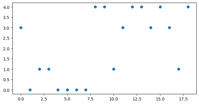
for sent_topics in doc_topics]At this point, it can be interesting to visualise the topic distributions to see if we can identify potential break points by visual inspection. We can plot a scatterplot over the above result using pyplot:
Window-based similarity calculation
The next steps are pretty straightforward, we will pass a sliding window over the above topic distribution to collect all topics that appear in each window.
from itertools import islice
def window(seq, n=3):
	it = iter(seq)
    result = tuple(islice(it, n))
    if len(result) == n:
    	yield result
    for elem in it:
    	result = result[1:] + (elem,)
        yield result
The function window performs a sliding window operation on the input sequence. We will apply it on the topics extracted from the previous step.
from itertools import chain
WINDOW_SIZE = 3
window_topics = window(top_k_topics, n=WINDOW_SIZE)
window_topics = [list(set(chain.from_iterable(window)))
				for window in window_topics]
where window_topics looks like the following, where each element represents a 3-sentence window
[[0, 1, 3],
 [0, 1],
 [0, 1],
 [0, 1],
 [0],
 [0],
 [0, 4],
 [0, 4],
 [1, 4],
 [1, 3, 4]]
Binarization
We would like to convert the above to a binary one-hot vector for cosine similarity calculation. Sklearn will allow us to do this easily.
from sklearn.preprocessing import MultiLabelBinarizer
binarizer = MultiLabelBinarizer(classes=range(N_TOPICS))
encoded_topic = binarizer.fit_transform(window_topics)
encoded_topic now contains the following, where a 1 for an index means that the corresponding topic appears at least once in that window. Thus, instead of bag-of-words, we compute bag-of-topics.
[[1, 1, 0, 1, 0],
 [1, 1, 0, 0, 0],
 [1, 1, 0, 0, 0],
 [1, 1, 0, 0, 0],
 [1, 0, 0, 0, 0],
 [1, 0, 0, 0, 0],
 [1, 0, 0, 0, 1],
 [1, 0, 0, 0, 1],
 [0, 1, 0, 0, 1],
 [0, 1, 0, 1, 1]]
Coherence score calculation
Using the above result, we simply have to compute a cosine similarity between adjacent pairs on windows. The similarity measures the coherence between two windows of text and a low value indicates a possible point of topic shift.
from sklearn.metrics.pairwise import cosine_similarity
coherence_scores = [cosine_similarity([pair[0]], [pair[1]])[0][0]
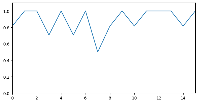
for pair in zip(encoded_topic, encoded_topic[1:])]We can visualise it as a line plot, where the x-axis represents a boundary index and y axis denotes the coherence score between two pairs of sliding windows that go over that boundary.
Computing Depth Scores
In principle, we are interested in the local minimal of the above plot. However, we need a way to quantify the depth of these minima in order to differentiate significant topic shifts from minor ones.
We quantify this depth via a new measure called the depth score. This measures how deep or shallow a minima is compared to others. This depth corresponds directly with how strongly the topic changed between two adjacent sentences.
Here, we will use the version of the depth score formula from the topic tiling paper.

To understand the above formula, we need to refer to the coherence score diagram above. p refers to the index of the boundary we wish to calculate the depth for, in this case p=7.
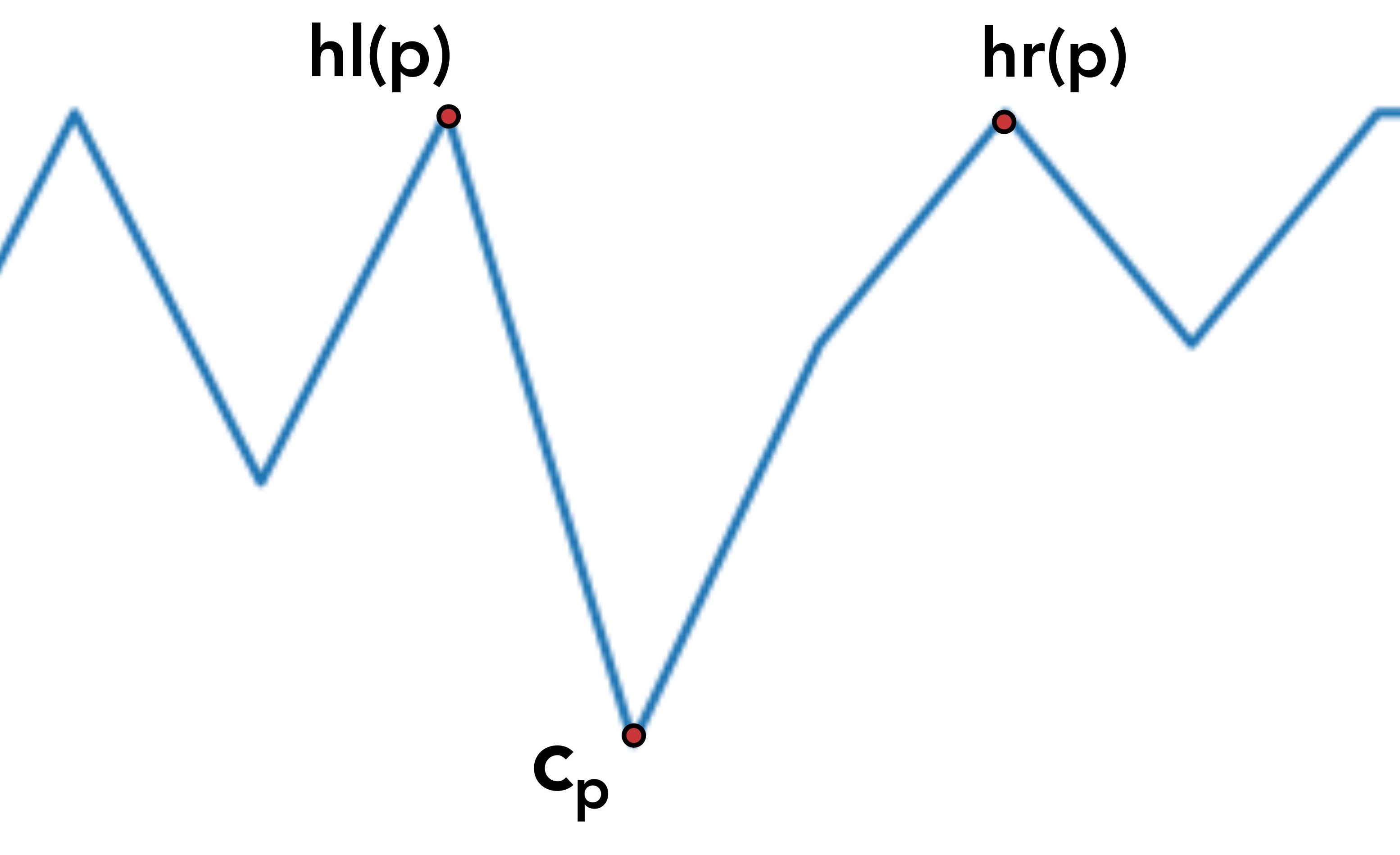
c_p is simply the coherence score at point p
hl is a function that takes a point p as input and returns the coherence score for the leftmost index where the score keeps increasing consecutively. hr does the same but returns the rightmost such index.
Thus, given a valley whose deepest point is at point p, hl(p) and hr(p) will return the height of the edges of that valley and c_p is the height of the lowest point.
Given a sequence of scores l and an index i, the function climb will return either hl(i) or hr(i)
def climb(seq, i, mode='left'):
    if mode == 'left':
        while True:
            curr = seq[i]
            if i == 0:
                return curr
            i = i-1
            if not seq[i] > curr:
                return curr
    if mode == 'right':
        while True:
            curr = seq[i]
            if i == (len(seq)-1):
                return curr
            i = i+1
            if not seq[i] > curr:
                return curr
Using the function above, we can apply the depth score formula to calculate the depths for each point in an input sequence. get_depths performs this operation.
def get_depths(scores):
    depths = []
    for i in range(len(scores)):
        score = scores[i]
        l_peak = climb(scores, i, mode='left')
        r_peak = climb(scores, i, mode='right')
        depth = 0.5 * (l_peak + r_peak - (2*score))
        depths.append(depth)
    return np.array(depths)
We run it as
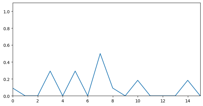
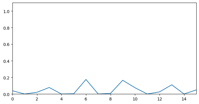
depth_scores = get_depths(coherence_scores)This will return the following depth score sequence, we notice that the valleys have been replaced by peaks and most of the other information in the sequence has been filtered out. A plot of depths_scores is as follows.
Removing plateaus from depth scores
A problem with the above scores is that some valleys tend to be be relatively wider, resulting in multiple points with high depth close to each other in a plateau shape. This has a chance to create multiple segments that are very close to each other.
To avoid this, we sharpen the plateaus by applying a local maxima filter. For each point, we only keep it if it is a local maxima of its adjacent points. The scipy routine argrelmax allows us to do this.
from scipy.signal import argrelmax

def get_local_maxima(depth_scores, order=1):
     maxima_ids = argrelmax(depth_scores, order=order)[0]
     filtered_scores = np.zeros(len(depth_scores))
     filtered_scores[maxima_ids] = depth_scores[maxima_ids]
     return filtered_scores
We run it as
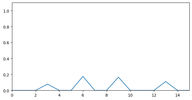
filtered_scores = get_local_maxima(depths_scores, order=1)A plot of filtered_topic gives:
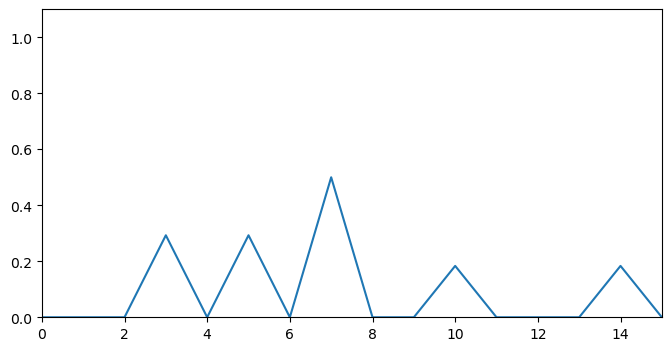
After applying the above filter, we notice that a lot of noise has been removed and the peaks are sharper, removing ambiguity in selecting segmentation candidates.
Computing threshold
At this point we could set an arbitrary threshold value and simply apply that to select segmentation points. However, threshold selection can be difficult as there is no meaning to the scale of the scores calculated so far.
The TextTiling paper described an approach to automatically calculate the optimal threshold by using the mean and standard deviation of the depth scores.
threshold = mean(depths) - std(depths) / 2
The following function will calculate the threshold automatically using the above equation:
def compute_threshold(scores):
     s = scores[np.nonzero(scores)]
     threshold = np.mean(s) - (np.std(s) / 2)
     # threshold = np.mean(s) - (np.std(s))
     return threshold
and we apply it as
threshold = compute_threshold(filtered_scores)Running above function on the above scores results in a threshold value of 0.2327
Selecting Segments
We can get the segment ids by using the above threshold on the filtered depth scores.
def get_threshold_segments(scores, threshold=0.1):
     segment_ids = np.where(scores >= threshold)[0]
     return segment_ids
The above function is applied to get the segmented ids
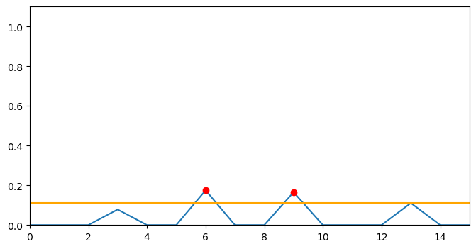
segment_ids = get_threshold_segments(filtered_scores, threshold)The results look like this:
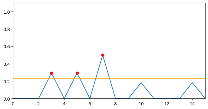
array([3, 5, 7])We can also plot the threshold and selected segments. The yellow line represents the threshold and the red dots represent the selected segments with highest topic shift.
Applying to text
Since the above ids represent segment gaps for adjacent windows, we need to translate them back to sentence gap ids, for this we need to add the WINDOW_SIZE parameter we used previously.
segment_indices = segment_ids + WINDOW_SIZEsegment_indices now contains
array([ 6, 8, 10])
Finally, we will convert these ids to index slices to apply to the original sentences
segment_indices = [0] + segment_indices.tolist() + [len(sents)]
slices = list(zip(segment_indices[:-1], segment_indices[1:]))
This returns
[(0, 6), (6, 8), (8, 10), (10, 19)]
Now we can simply apply these slices to our original document
segmented = [sents[s[0]: s[1]] for s in slices]The results can be seen in this text file. The SEGMENT tag represents the breakpoints.
Analysis
The text is broken into 4 segments based on the topic model, upon manual inspection we notice that the segment do correspond to topic shifts somewhat.
- The first segment gives an overview of the story.
- The second segments talks mainly about the new judges.
- The third segment details a quote by one of the judges.
- The fourth segments covers the remaining story.
Higher quality segments could be extracted via this method by training a topic model on a large news corpus with a higher number of topics.
b) LLM Based Segmentation
In the previous approach we used a topic model to identify similarities between text segments. A limitation of this approach is that a topic model has to be trained on a domain-specific corpus beforehand. Even then, the quality of the generated topics may vary on each run and the model may not work well on texts from different domains.
Large Language Models (LLMs) like BERT can provide an alternative approach to text similarity computation. These are generally pre-trained on a large text corpus covering various domains and can thus be used out-of-the-box for various tasks.
We can create a variation of topic-tiling where we use an LLM for the similarity computation part while keeping everything else the same.
Initialising the model
The SentenceTransformer module provides a simple interface to access various large language models and apply them directly to sentence units.
from sentence_transformers import SentenceTransformer
MODEL_STR = "sentence-transformers/all-MiniLM-L6-v2"
model = SentenceTransformer(MODEL_STR)
The model all-MiniLM-L6-v2 is a variation of Microsoft’s MiniLM model which is further fine-tuned on a large sentence-pairs dataset. According to the sentence transformers documentation, it is suitable for semantic search and is intended to be used for sentences and short paragraphs. Seems like a good match for our task.
Applying the Sliding Window
Since there is no model training step, we can proceed directly to sliding window computation. Since MiniLM uses its own tokeniser, we can also skip the tokenisation and preprocessing steps.
In the following code we apply the window function directly to the raw sentences.
WINDOW_SIZE = 3
window_sent = list(window(sents, WINDOW_SIZE))
window_sent = [' '.join([sent.text for sent in window]) for window in window_sent]
Each element of window_sent now contains a sequence of sentences of length WINDOW_SIZE
Model Inference
We can encode the windowed sentences directly using MiniLM
encoded_sent = model.encode(window_sent)encoded_sent is now a vector of shape (17, 384) where 17 is the number of windows and 384 is the dimensionality of the large language model’s vector space.
Coherence Score Computation
We can directly use cosine similarity on the encoded sentences to compute the coherence scores.
coherence_scores = [cosine_similarity([pair[0]], [pair[1]])[0][0] for pair in zip(encoded_sent, encoded_sent[1:])]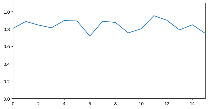
Depth Score Computation
Now we can compute the depth scores
depth_scores = get_depths(coherence_scores)
Filtering the Depth Scores
The filtering step is also the same as before
filtered_scores = get_local_maxima(depths_topic, order=1)
Thresholding Step
Finally, we can compute the threshold and generate segments.
threshold = compute_threshold(filtered_scores) segments_ids = get_threshold_segments(filtered_scores, threshold)
This time we got a threshold value of 0.1127
We can generate a plot summarising the thresholding step.
Segmentation Output
We can repeat the previous steps to generate the segmented sentences. The final output can be seen on this file. There are some minor differences from the topic segmentation result. The first and third segments are pretty generic but the second segment seems to focus on details about a certain court building in New Orleans.
Model Evaluation
So far, we haven’t covered the numerical evaluation of the techniques described in this article. An easy way to evaluate topic segmentation is to attach two snippets from different articles together and then segment it using one of the previous approaches.
The algorithm can then be evaluated on its ability to identify the point where the article changes to a different one. More rigorous evaluation would require hand-annotated data however.
This article gives a good overview of some evaluation metrics for text segmentation as well as datasets in the research literature.
Conclusion
In this article I described an approach to text segmentation using topics models and LLMs. However, any other similarity function is also applicable as long as it can return a similarity value between pairs of texts.
In a later article I will cover hands-on evaluation of topic segmentation in detail.
Code and Interactive Demo
A notebook containing the code in this post can be accessed here.
An interactive demo is built using Streamlit is hosted here.